머신러닝 기초 수학 7 - Linear Regression
7. Linear Regression
<Linear Regression 참고>

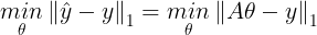
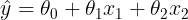
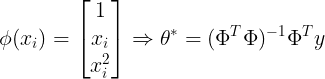
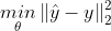
- ŷ과 실제 output인 y^(i)의 차에 합 또는 평균 낸 값을 최소로 내는 ω를 찾는 것
1) 선형회귀

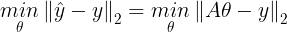
- 최소자승법 이용

<실습>
실습 1 : Linear Regression 실습
import numpy as np
import matplotlib.pyplot as plt
%matplotlib inline
x = np.array([0.1,0.4,0.7,1.2,1.3,1.7,2.2,2.8,3.0,4.0,4.3,4.4,4.9]).reshape(-1,1)
y = np.array([0.5,0.9,1.1,1.5,1.5,2.0,2.2,2.8,2.7,3.0,3.5,3.7,3.9]).reshape(-1,1)
plt.figure(figsize=(10,8))
plt.plot(x,y,'ko')
plt.title('Data',fontsize =15)
plt.xlabel('X',fontsize=15)
plt.ylabel('Y',fontsize=15)
plt.axis('equal')
plt.grid(alpha=0.3)
plt.xlim([0,5])
plt.show()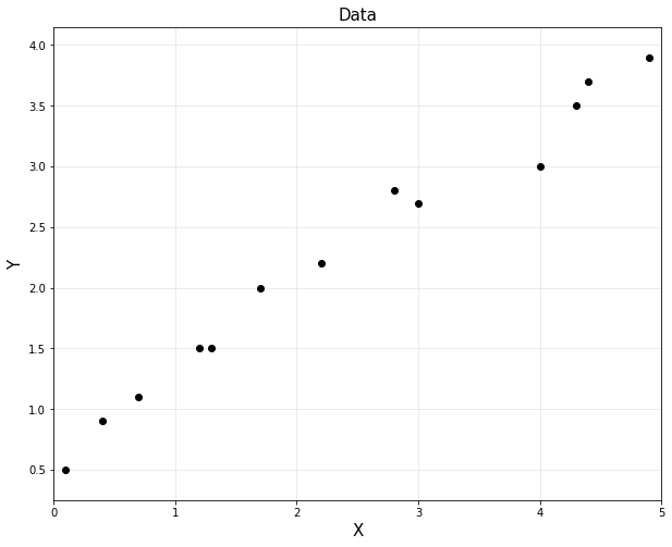
- 세타 구하기
import numpy as np
m = x.shape[0]
A = np.hstack([np.ones([m,1]),x])
A = np.hstack([x**0,x])
A = np.asmatrix(A)
theta = (A.T*A).I*A.T*A
print(A)


[[1.  0.1]
 [1.  0.4]
 [1.  0.7]
 [1.  1.2]
 [1.  1.3]
 [1.  1.7]
 [1.  2.2]
 [1.  2.8]
 [1.  3. ]
 [1.  4. ]
 [1.  4.3]
 [1.  4.4]
 [1.  4.9]]
- 직선 combine
plt.figure(figsize=(10,8))
plt.title('Regression',fontsize =15)
plt.xlabel('X',fontsize=15)
plt.ylabel('Y',fontsize=15)
plt.plot(x,y,'ko',label="data")

xp = np.arange(0,5,0.01).reshape(-1,1)
yp = theta[0,0]+theta[1,0]*xp
plt.plot(xp,reg.predict(xp), 'r',linewidth=2,label="regression")
plt.legend(fontsize =15)
plt.axis('equal')
plt.grid(alpha=0.3)
plt.xlim([0,5])
plt.show()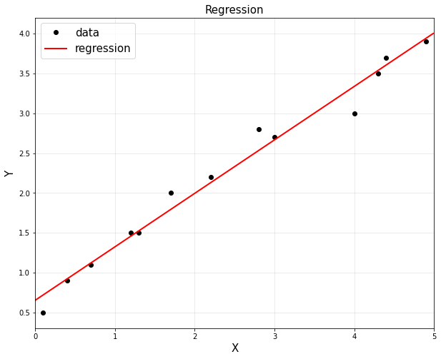
실습 2 : CVXPY를 이용한 최적화 솔루션
import cvxpy as cvx
theta1 = cvx.Variable([2,1])
obj = cvx.Minimize(cvx.norm(A*theta1 - y,1))  # theta 1
prob = cvx.Problem(obj,[])
result = prob.solve()
print('theta1:\n', theta1.value)

theta2 = cvx.Variable([2,1])
obj = cvx.Minimize(cvx.norm(A*theta2 - y, 2)) # theta 2
prob = cvx.Problem(obj,[])
result = prob.solve()
print('theta2:\n', theta2.value)


theta1:
 [[0.6258404 ]
 [0.68539899]]
theta2:
 [[0.65306531]
 [0.67129519]]
- 그래프 생성
plt.figure(figsize=(10,8))
plt.title('$L_1$ and $L_2$ Regression', fontsize =15)
plt.xlabel('X', fontsize = 15)
plt.ylabel('Y', fontsize = 15)
plt.plot(x,y,'ko',label="data")

xp = np.arange(0,5,0.01).reshape(-1,1)
yp1 = theta1.value[0,0] + theta1.value[1,0]*xp
yp2 = theta2.value[0,0] + theta2.value[1,0]*xp

plt.plot(xp,yp1, 'b', linewidth =2, label = '$L_1$')
plt.plot(xp,yp2, 'r', linewidth =2, label = '$L_2$')
plt.legend(fontsize = 15)
plt.axis('equal')
plt.xlim([0,5])
plt.grid(alpha=0.3)
plt.show()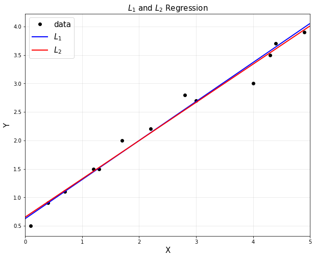
- L1과 L2의 outliers에 대한 차이는 분명하다
from sklearn import linear_model
import numpy as np
import matplotlib.pyplot as plt
import cvxpy as cvx
%matplotlib inline
x = np.array([0.1,0.4,0.7,1.2,1.3,1.7,2.2,2.8,3.0,4.0,4.3,4.4,4.9]).reshape(-1,1)
y = np.array([0.5,0.9,1.1,1.5,1.5,2.0,2.2,2.8,2.7,3.0,3.5,3.7,3.9]).reshape(-1,1)
x = np.vstack([x,np.array([0.5,3.8]).reshape(-1,1)])
y = np.vstack([y,np.array([3.9,0.3]).reshape(-1,1)])
A = np.hstack([x**0, x])
A = np.asmatrix(A)

theta1 = cvx.Variable([2,1])
obj1 = cvx.Minimize(cvx.norm(A*theta1 - y, 1))
prob1 = cvx.Problem(obj1).solve()

theta2 = cvx.Variable([2,1])
obj2 = cvx.Minimize(cvx.norm(A*theta2 - y, 2))
prob2 = cvx.Problem(obj2).solve()

plt.figure(figsize = (10,8))
plt.plot(x,y,'ko',label='data')
plt.title('$L_1$ and $L_2$ Regression w/ Outliers', fontsize = 15)
plt.xlabel('X', fontsize = 15)
plt.ylabel('Y', fontsize = 15)

xp = np.arange(0,5,0.01).reshape(-1,1)
yp1 = theta1.value[0,0] + theta1.value[1,0]*xp
yp2 = theta2.value[0,0] + theta2.value[1,0]*xp

plt.plot(xp,yp1,'b', linewidth=2,label = '$L_1$')
plt.plot(xp,yp2,'r', linewidth=2,label = '$L_2$')
plt.axis('scaled')
plt.xlim([0,5])
plt.legend(fontsize = 15, loc = 5)
plt.grid(alpha = 0.3)
plt.show()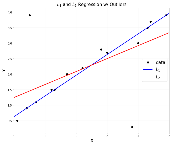
실습 3 : CVXPY를 이용한 최적화 솔루션 => 위와 동일 결과
from sklearn import linear_model
import numpy as np
import matplotlib.pyplot as plt
%matplotlib inline
x = np.array([0.1,0.4,0.7,1.2,1.3,1.7,2.2,2.8,3.0,4.0,4.3,4.4,4.9]).reshape(-1,1)
y = np.array([0.5,0.9,1.1,1.5,1.5,2.0,2.2,2.8,2.7,3.0,3.5,3.7,3.9]).reshape(-1,1)
reg = linear_model.LinearRegression()
reg.fit(x,y)
reg.coef_ # theta 1 : array([[0.67129519]])  계수
reg.intercept_ # theta 0 : array([0.65306531])   바이어스
plt.figure(figsize=(10,8))
plt.title('$L_1$ and $L_2$ Regression', fontsize =15)
plt.xlabel('X', fontsize = 15)
plt.ylabel('Y', fontsize = 15)
plt.plot(x,y,'ko',label="data")
# sklearn은 xp, reg.predict(xp)의 xp를 기입하지 않아도 실행된다.
plt.plot(xp, reg.predict(xp), 'r', linewidth = 2, label = "regression")
plt.legend(fontsize = 15)
plt.axis('equal')
plt.xlim([0,5])
plt.grid(alpha=0.3)
plt.show()
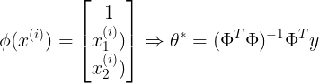
2) 다중 선형 회귀
<1> Linear Regression : multivariate data
import numpy as np
import matplotlib.pyplot as plt
%matplotlib inline
from mpl_toolkits.mplot3d import Axes3D

n = 200
x1 = np.random.randn(n,1)
x2 = np.random.randn(n,1)
noise = 0.5*np.random.randn(n,1);
y = 2+1*x1+3*x2 + noise

fig = plt.figure(figsize = (10,8))
ax = fig.add_subplot(1,1,1,projection = '3d')
ax.set_title('Generated Data', fontsize = 15)
ax.set_xlabel('$x_1$', fontsize = 15)
ax.set_ylabel('$x_2$', fontsize = 15)
ax.set_zlabel('Y', fontsize = 15)
ax.scatter(x1,x2,y,marker = '.', label = 'Data')
ax.view_init(30,0)
plt.legend(fontsize=15)
plt.show()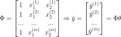
A = np.hstack([x1**0,x1,x2])
A = np.asmatrix(A) # basis function
theta = (A.T*A).I*A.T*y
x1, x2 = np.meshgrid(np.arange(np.min(x1), np.max(x1),0.5),
                     np.arange(np.min(x2), np.max(x2),0.5))
YP = theta[0,0] + theta[1,0]*x1 + theta[2,0]*x2

fig = plt.figure(figsize = (10,8))
ax = fig.add_subplot(1,1,1,projection = '3d')
ax.set_title('Regression', fontsize = 15)
ax.set_xlabel('$x_1$', fontsize = 15)
ax.set_ylabel('$x_2$', fontsize = 15)
ax.set_zlabel('Y', fontsize = 15)
ax.scatter(x1, x2, y, marker = '.', label = 'Data')
ax.plot_wireframe(x1,x2,YP,color = 'k', alpha = 0.3, label = 'Regression Plane')
plt.legend(fontsize = 15)
plt.show()
<2> Nonlinear Regression : multivariate data

import numpy as np
import matplotlib.pyplot as plt
%matplotlib inline
from mpl_toolkits.mplot3d import Axes3D

n = 100
x = -5 + 15*np.random.rand(n,1)
noise = 10*np.random.randn(n,1)
y = 10 + 1*x+2*x**2+noise

A = np.hstack([x**0, x, x**2])
A = np.asmatrix(A)
theta = (A.T*A).I*A.T*y
print('theta:\n', theta)

xp = np.linspace(np.min(x), np.max(x))
yp = theta[0,0] + theta[1,0]*xp + theta[2,0]*xp **2
plt.figure(figsize = (10,8))
plt.plot(x,y,'o',markersize = 4, label='actual')
plt.plot(xp,yp,'r',linewidth=2, label='estimated')
plt.title('Nonlinear regression', fontsize = 15)
plt.xlabel('X', fontsize = 15)
plt.ylabel('Y', fontsize = 15)
plt.xlim([np.min(x),np.max(x)])
plt.grid(alpha = 0.3)
plt.legend(fontsize = 15)
plt.show()


theta:
 [[9.31695129]
 [1.13434779]
 [2.04402726]]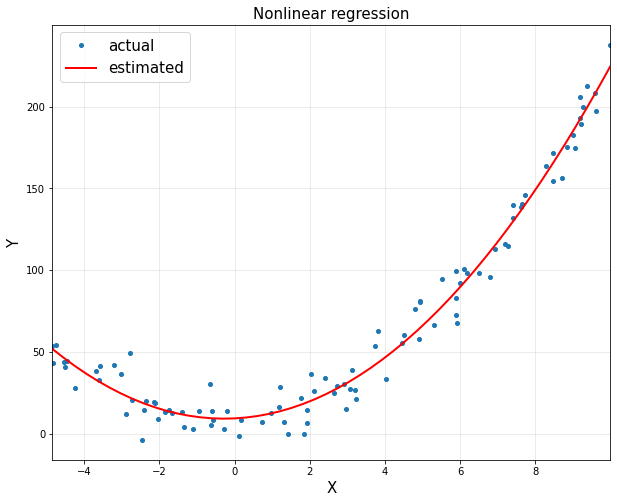
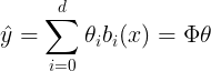
<3> Polynomial functions
- Function Approximation 관점 : target에 가장 근사하게 접근하는 관점
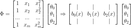
- 선형 조합으로 대상 함수를 근사화
import numpy as np
import matplotlib.pyplot as plt
%matplotlib inline
from mpl_toolkits.mplot3d import Axes3D

d = 6
xp = np.arange(-1,1,0.01).reshape(-1,1)
polybasis = np.hstack([xp**i for i in range(d)])

plt.figure(figsize = (10,8))
for i in range(d):
  plt.plot(xp, polybasis[:,i], label='$x^{}$'.format(i))
plt.title('Polynomial basis', fontsize = 15)
plt.xlabel('X', fontsize = 15)
plt.ylabel('Y', fontsize = 15)
plt.axis([-1,1,-1.1,1.1])
plt.legend(fontsize= 15)
plt.grid(alpha = 0.3)
plt.show()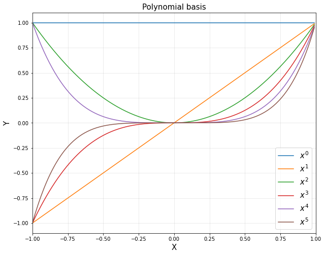
- Regression + Polynomial basis
import numpy as np
import matplotlib.pyplot as plt
%matplotlib inline
from mpl_toolkits.mplot3d import Axes3D

n = 100
x = -5 + 15*np.random.rand(n,1)
noise = 10*np.random.randn(n,1)
y = 10 + 1*x+2*x**2+noise

xp = np.arange(np.min(x), np.max(x), 0.01).reshape(-1,1)
d = 3
polybasis = np.hstack([xp**i for i in range(d)])
polybasis = np.asmatrix(polybasis)
A = np.hstack([x**i for i in range(d)])
A = np.asmatrix(A)

theta = (A.T*A).I*A.T*y

yp = polybasis*theta

plt.figure(figsize = (10,8))
plt.plot(x,y,'o',label = 'Data')
plt.plot(xp,yp, label='Polynomial')
plt.title('Regression with Polynomial basis', fontsize = 15)
plt.xlabel('X', fontsize = 15)
plt.ylabel('Y', fontsize = 15)
plt.grid(alpha = 0.3)
plt.legend(fontsize= 15)
plt.show()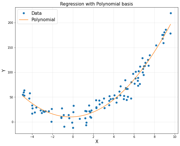
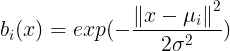
<4> RBF functions
import numpy as np
import matplotlib.pyplot as plt
%matplotlib inline
from mpl_toolkits.mplot3d import Axes3D

d = 9
u = np.linspace(-1,1,d)
sigma = 0.2
xp = np.arange(-1,1,0.01).reshape(-1,1)
rbfbasis = np.hstack([np.exp(-(xp-u[i])**2/(2*sigma**2)) for i in range(d)])

plt.figure(figsize = (10,8))
for i in range(d):
  plt.plot(xp, rbfbasis[:,i], label='$\mu = ()$'.format(u[i]))
plt.title('RBF basis', fontsize = 15)
plt.xlabel('X', fontsize = 15)
plt.ylabel('Y', fontsize = 15)
plt.axis([-1,1,-0.1,1.1])
plt.legend(loc = 'lower right', fontsize= 15)
plt.grid(alpha = 0.3)
plt.show()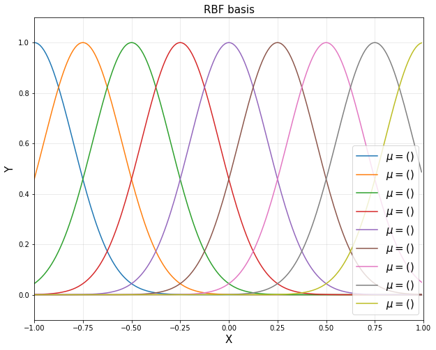
- Regression + RBF basis
import numpy as np
import matplotlib.pyplot as plt
%matplotlib inline
from mpl_toolkits.mplot3d import Axes3D

n = 100
x = -5 + 15*np.random.rand(n,1)
noise = 10*np.random.randn(n,1)
y = 10 + 1*x+2*x**2+noise

xp = np.arange(np.min(x), np.max(x), 0.01).reshape(-1,1)

d = 9
u = np.linspace(np.min(x), np.max(x))
sigma = 10

rbfbasis = np.hstack([np.exp(-(xp-u[i])**2/(2*sigma**2)) for i in range(d)])
rbfbasis = np.asmatrix(rbfbasis)

A = np.hstack([np.exp(-(x-u[i])**2/(2*sigma**2)) for i in range(d)])
A = np.asmatrix(A)
theta = (A.T*A).I*A.T*y
yp = rbfbasis*theta

plt.figure(figsize = (10,8))
plt.plot(x,y,'o', label = 'Data')
plt.plot(xp, yp, label = 'RBF')
plt.title('Regression with RBF basis', fontsize = 15)
plt.xlabel('X', fontsize = 15)
plt.ylabel('Y', fontsize = 15)
plt.legend(fontsize= 15)
plt.grid(alpha = 0.3)
plt.show()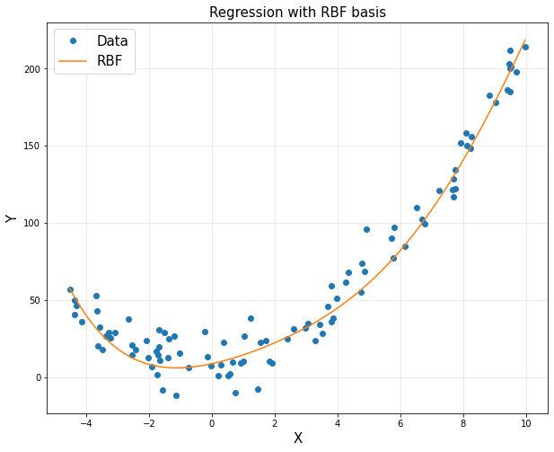
3) 과적합
<1> Nonlinear Regression
import numpy as np
import matplotlib.pyplot as plt
%matplotlib inline

n = 10
x = np.linspace(-4.5,4.5,10).reshape(-1,1)
y = np.array([0.9819,0.7973,1.9737,0.1838,1.3180,-0.8361,-0.6591,-2.4701,-2.8122,-6.2512]).reshape(-1,1)
d = [1,3,5,9]
RSS = []
plt.figure(figsize = (12,10))
plt.suptitle('Nonlinear Regression', fontsize = 15)

A = np.hstack([x**0, x])
A = np.asmatrix(A)
theta = (A.T*A).I*A.T*y


for k in range(4):
  xp = np.arange(-4.5,4.5,0.01).reshape(-1,1)
  yp = theta[0,0] + theta[1,0]*xp
  A = np.hstack([x**i for i in range(d[k]+1)])
  polybasis = np.hstack([xp**i for i in range(d[k]+1)])

  A = np.asmatrix(A)
  polybasis = np.asmatrix(polybasis)
  theta = (A.T*A).I*A.T*y
  yp = polybasis*theta

  RSS.append(np.linalg.norm(y-A*theta, 2 )**2)

  plt.subplot(2,2,k+1)
  plt.plot(x,y,'o')
  plt.plot(xp,yp)
  plt.axis([-5,5,-12,6])
  plt.title('degree = {}'.format(d[k]))
  plt.grid(alpha=0.3)
plt.show()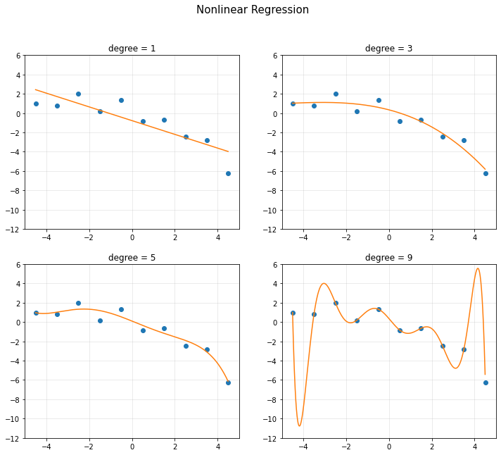
- RSS(Loss) : Residual Sum of Squares
- 에러를 제곱한 형태를 뜻한다.

- 모델의 복잡도 complexity가 커지면 RSS가 줄어든다.
- 위 식이 항상 best는 아니다.
import numpy as np
import matplotlib.pyplot as plt
%matplotlib inline

n = 10
x = np.linspace(-4.5,4.5,10).reshape(-1,1)
y = np.array([0.9819,0.7973,1.9737,0.1838,1.3180,-0.8361,-0.6591,-2.4701,-2.8122,-6.2512]).reshape(-1,1)
d = [1,3,5,9]
RSS = []
plt.figure(figsize = (12,10))
plt.suptitle('Nonlinear Regression', fontsize = 15)

A = np.hstack([x**0, x])
A = np.asmatrix(A)
theta = (A.T*A).I*A.T*y


for k in range(4):
  xp = np.arange(-4.5,4.5,0.01).reshape(-1,1)
  yp = theta[0,0] + theta[1,0]*xp
  A = np.hstack([x**i for i in range(d[k]+1)])
  polybasis = np.hstack([xp**i for i in range(d[k]+1)])

  A = np.asmatrix(A)
  polybasis = np.asmatrix(polybasis)
  theta = (A.T*A).I*A.T*y
  yp = polybasis*theta

  RSS.append(np.linalg.norm(y-A*theta, 2 )**2)


plt.figure(figsize = (10,8))
plt.stem(d,RSS, label = 'RSS')
plt.title('Residual Sum of Squares', fontsize = 15)
plt.xlabel('degree',fontsize = 15)
plt.ylabel('RSS', fontsize = 15)
plt.legend(fontsize = 15)
plt.grid(alpha = 0.3)
plt.show()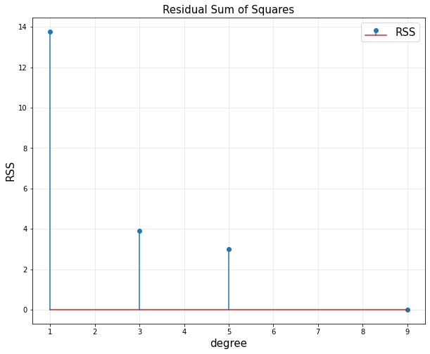
<Rich Representation>
- 문제점 : input data에선 에러가 작지만 근처에선 에러가 크고 training data에선 에러가 작지만, 학습 시 사용하지 않았던 testing data에선 에러가 크다.
- RBF Function Overfitting
import numpy as np
import matplotlib.pyplot as plt
%matplotlib inline

n = 10
x = np.linspace(-4.5,4.5,10).reshape(-1,1)
y = np.array([0.9819,0.7973,1.9737,0.1838,1.3180,-0.8361,-0.6591,-2.4701,-2.8122,-6.2512]).reshape(-1,1)

xp = np.arange(-4.5,4.5,0.01).reshape(-1,1)
d = [2,4,6,10]
plt.figure(figsize = (12,10))
sigma = 5

for k in range(4):
  u = np.linspace(-4.5,4.5,d[k])
  A = np.hstack([np.exp(-(x - u[i])**2/(2*sigma**2)) for i in range(d[k])])

  rbfbasis = np.hstack([np.exp(-(xp-u[i])**2/(2*sigma**2)) for i in range(d[k])])
  A = np.asmatrix(A)
  rbfbasis = np.asmatrix(rbfbasis)

  theta = (A.T*A).I*A.T*y
  yp = rbfbasis*theta
  plt.subplot(2,2,k+1)
  plt.plot(x,y,'o')
  plt.plot(xp,yp)
  plt.axis([-5,5,-12,6])
  plt.title('num RBFs = {}'.format(d[k]), fontsize = 10)
  plt.grid(alpha = 0.3)

plt.suptitle('Nonlinear Regression with RBF Functions', fontsize = 15)
plt.show()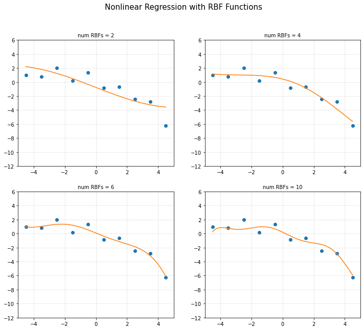
- 정규화 (릿지, 라쏘)를 이용한 과적합 문제를 해결할 수 있다.
4) 정규화
- training data를 최소화하는게 아니라 generalization 에러를 최소화 해야한다.
(1) 의도적으로 표현을 못하게 한다. (Polynomial은 차수를 줄이고, RBF는 개수를 줄임) or band width를 크게
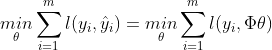
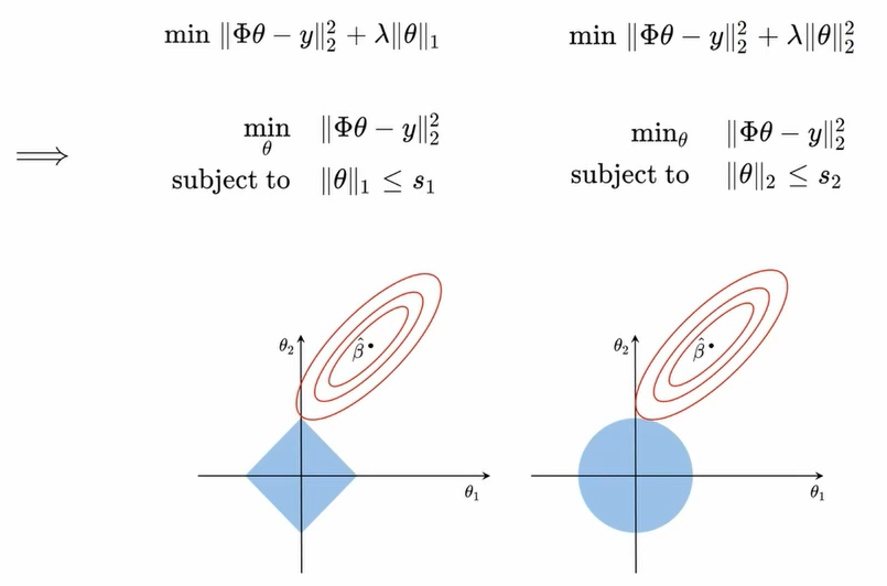
(2)

에서 파라미터를 강제로 갖게 만든다 => Regularization (정규화)


import cvxpy as cvx
import numpy as np
import matplotlib.pyplot as plt

x = np.linspace(-4.5,4.5,10).reshape(-1,1)
y = np.array([0.9819, 0.7973, 1.9737,0.1838,1.3180, -0.8361, -0.6591, -2.4701, -2.8122, -6.2512]).reshape(-1,1)
xp = np.arange(-4.5,4.5,0.01).reshape(-1,1)
d = 10
u = np.linspace(-4.5,4.5,d)
sigma = 1
rbfbasis = np.hstack([np.exp(-(xp-u[i])**2/(2*sigma**2)) for i in range(d)])
A = np.hstack([np.exp(-(x-u[i])**2/(2*sigma**2)) for i in range(d)])

rbfbasis = np.asmatrix(rbfbasis)
A = np.asmatrix(A)

lamb = 0.1
theta = cvx.Variable([d,1])
obj = cvx.Minimize(cvx.sum_squares(A*theta - y) + lamb * cvx.sum_squares(theta))
prob = cvx.Problem(obj, []).solve()

yp = rbfbasis*theta.value
plt.figure(figsize = (10,8))
plt.plot(x,y,'o',label = 'Data')
plt.plot(xp,yp,label = 'Overfitted')
plt.title('(Overfitted) Regression, fontsize = 15')
plt.xlabel('X', fontsize = 15)
plt.ylabel('Y', fontsize = 15)
plt.axis([-5,5,-12,6])
plt.legend(fontsize = 15)
plt.grid(alpha = 0.3)
plt.show()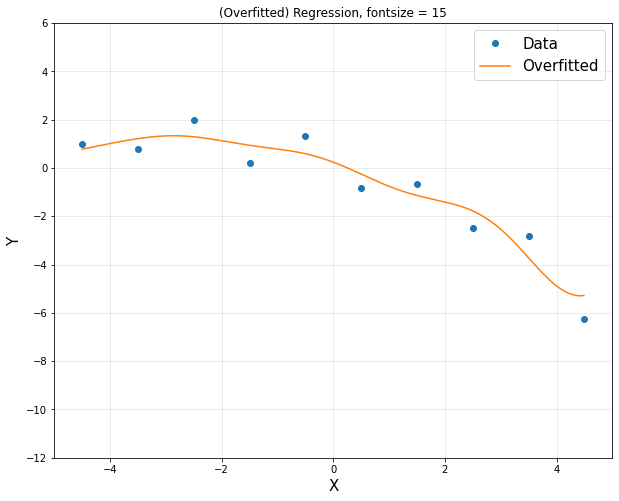
<Ridge vs Lasso>
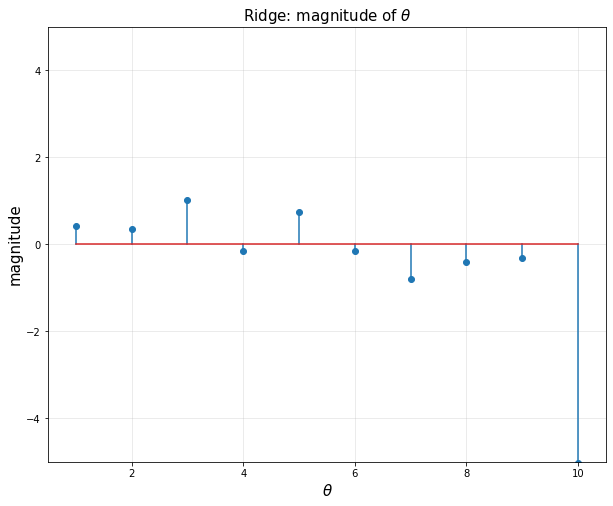
- Ridge
- 0이 없다
- bi를 10개 다 써야한다.
- 세타 값을 작게 만든다.
- Lasso
- Feature selecting 사용가능
- Sparsity
- 많은 변수가 0의 값을 가진다. bi를 4개 쓰고 세타 값을 0으로 만든다.
import cvxpy as cvx
import numpy as np
import matplotlib.pyplot as plt

x = np.linspace(-4.5,4.5,10).reshape(-1,1)
y = np.array([0.9819, 0.7973, 1.9737,0.1838,1.3180, -0.8361, -0.6591, -2.4701, -2.8122, -6.2512]).reshape(-1,1)
xp = np.arange(-4.5,4.5,0.01).reshape(-1,1)
d = 10
u = np.linspace(-4.5,4.5,d)
sigma = 1
rbfbasis = np.hstack([np.exp(-(xp-u[i])**2/(2*sigma**2)) for i in range(d)])
A = np.hstack([np.exp(-(x-u[i])**2/(2*sigma**2)) for i in range(d)])

rbfbasis = np.asmatrix(rbfbasis)
A = np.asmatrix(A)

lamb = 0.1
theta = cvx.Variable([d,1])
obj = cvx.Minimize(cvx.sum_squares(A*theta - y) + lamb * cvx.sum_squares(theta))
prob = cvx.Problem(obj, []).solve()
yp = rbfbasis*theta.value

plt.figure(figsize = (10,8))
plt.title(r'Ridge: magnitude of $\theta$', fontsize = 15)
plt.xlabel(r'$\theta$', fontsize = 15)
plt.ylabel('magnitude', fontsize = 15)
plt.stem(np.linspace(1,10,10).reshape(-1,1), theta.value)
plt.xlim([0.5,10.5])
plt.ylim([-5,5])
plt.grid(alpha = 0.3)
plt.show()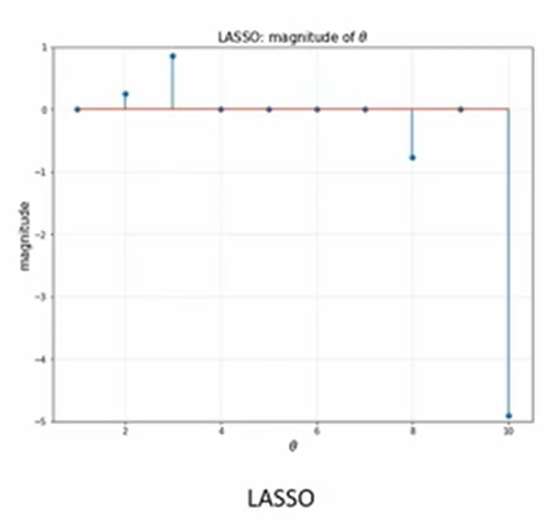
5) Regression 예시
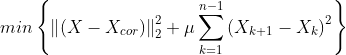
<De-noising signal : 노이즈 줄이기>
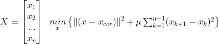
- 시그널은 노이즈에 비해 빠르게 변화하지 않고 이웃한 신호들의 크기는 유사하다
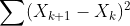
- min{ how much x deviates from Xcor + Penalize rapid changes of X}

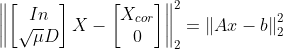
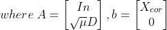
- mu : 첫 번째 텀과 두 번째 텀의 상대적 weight x의 smoothness를 컨트롤한다.
- 실습을 위한 노이즈 그래프 생성
import numpy as np
import matplotlib.pyplot as plt
import cvxpy as cvx
%matplotlib inline

n = 200
t = np.arange(n).reshape(-1,1)
x = 0.5 * np.sin((2*np.pi/n)*t)*(np.sin(0.01*t))
x_cor = x + 0.05*np.random.randn(n,1)

plt.figure(figsize = (10,8))
plt.subplot(2,1,1)
plt.plot(t,x,'-',linewidth = 2)
plt.axis([0,n,-0.6,0.6])
plt.xticks([])
plt.title('original signal', fontsize = 15)
plt.ylabel('$x_{original}$', fontsize = 15)
plt.subplot(2,1,2)
plt.plot(t, x_cor, '-', linewidth = 1)
plt.axis([0,n,-0.6,0.6])
plt.title('corrupted signal', fontsize = 15)
plt.xlabel('n', fontsize = 15)
plt.ylabel('$x_{corrupted}$', fontsize = 15)
plt.show()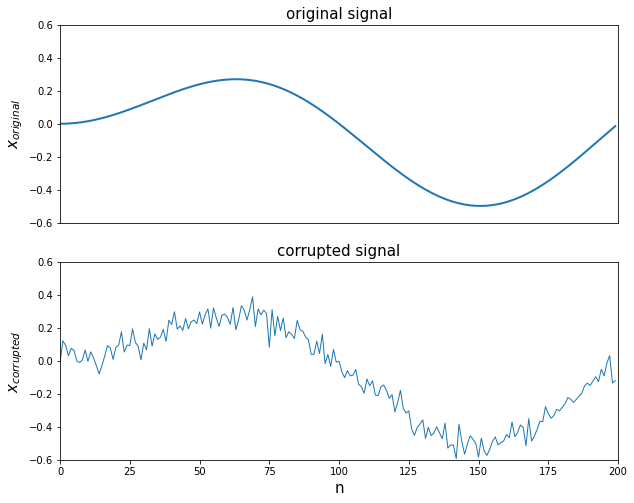

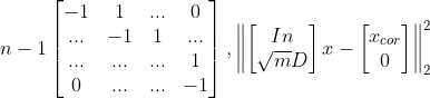
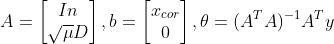
- smoothing과 mu의 상관관계

import numpy as np
import matplotlib.pyplot as plt
import cvxpy as cvx
n = 200
t = np.arange(n).reshape(-1,1)
x = 0.5 * np.sin((2*np.pi/n)*t)*(np.sin(0.01*t))
x_cor = x+0.05 * np.random.randn(n,1)
mu = [0,10,100]
D = np.zeros([n-1,n])
D[:,0:n-1] = D[:,0:n-1] - np.eye(n-1)
D[:,1:n] = D[:,1:n] + np.eye(n-1)

for i in range(len(mu)):
  A = np.vstack([np.eye(n), np.sqrt(mu[i])*D])
  b = np.vstack([x_cor, np.zeros([n-1,1])])
  A = np.asmatrix(A)
  b = np.asmatrix(b)
  x_reconst = (A.T*A).I*A.T*b
  plt.subplot(3,1,i+1)
  plt.plot(t,x_cor,'-',linewidth=1,alpha=0.3)
  plt.plot(t,x_reconst, 'r', linewidth =2)
  plt.ylabel('$\mu = {}$'.format(mu[i]), fontsize = 15)
plt.show()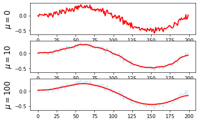


mu = 100
x_reconst = cvx.Variable([n,1])
obj = cvx.Minimize(cvx.sum_squares(x_reconst - x_cor) + mu *cvx.sum_squares(D*x_reconst))
prob = cvx.Problem(obj).solve()

plt.figure(figsize = (10,4))
plt.plot(t, x_cor, '-', linewidth=1, alpha=0.3, label='corrupted')
plt.plot(t, x_reconst.value, 'r', linewidth =2, label = 'reconstructed')
plt.title('$\mu = {}$'.format(mu), fontsize = 15)
plt.legend(fontsize = 12)
plt.show()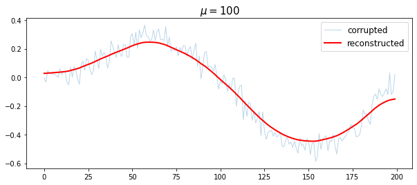
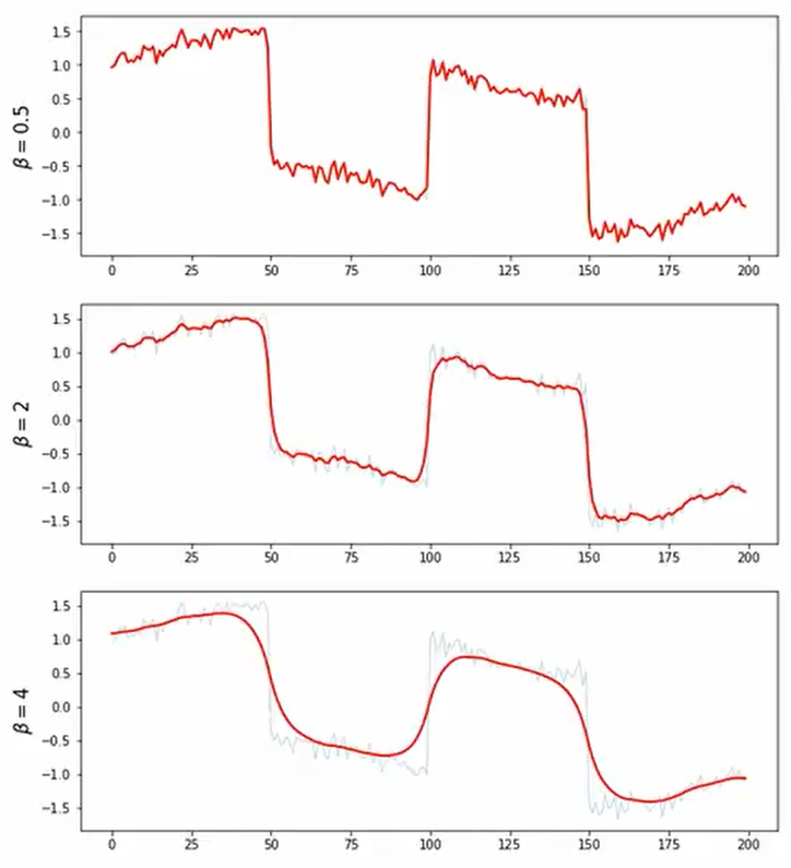
- 일부 그래프에선 L2 norm을 사용하면 노이즈를 복원하기 어렵다. 노이즈가 아닌부분도 노이즈로 인식하기 때문이다.
import numpy as np
import matplotlib.pyplot as plt
import cvxpy as cvx
n = 200
t = np.arange(n).reshape(-1,1)
x = 0.5 * np.sin((2*np.pi/n)*t)*(np.sin(0.01*t))
x_cor = x+0.05 * np.random.randn(n,1)
plt.figure(figsize = (10,12))
beta = [0.5,2,4]
for i in range(len(beta)):
  x_reconst = cvx.Variable([n,1])
  obj = cvx.Minimize(cvx.norm(x_reconst[1:n] - x_reconst[0:n-1],2))
  const = [cvx.norm(x_reconst - x_cor, 2) <= beta[i]]
  prob = cvx.Problem(obj,const).solve()
  plt.subplot(len(beta), 1, i+1)
  plt.plot(t,x_cor, linewidth =1, alpha =0.3)
  plt.plot(t, x_reconst.value, 'r', linewidth =2)
  plt.ylabel(r'$\beta = {}$'.format(beta[i]), fontsize = 15)
plt.show()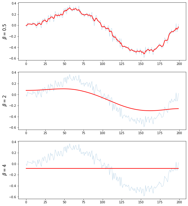
plt.figure(figsize = (10,12))
gammas = [0,2,7]
for i in range(len(gammas)):
  x_reconst = cvx.Variable([n,1])
  obj = cvx.Minimize(cvx.norm(x_reconst - x_cor, 2) + gammas[i]*cvx.norm(D*x_reconst, 2))
  '''
  제약조건 L2norm
  beta = 0.8
  obj = cvx.Minimize(cvx.norm(D*x_reconst, 2))
  const = [cvx.norm(x_reconst - x_cor, 2) <= beta]
  plt.figure(figsize = (10,4))
  '''
  prob = cvx.Problem(obj).solve()
  plt.subplot(3,1,i+1)
  plt.plot(t,x_cor, '-', linewidth = 1, alpha = 0.3)
  plt.plot(t,x_reconst.value, 'r', linewidth = 2)
  plt.ylabel('$ \gamma = {}$'.format(gammas[i]), fontsize = 15)
plt.show()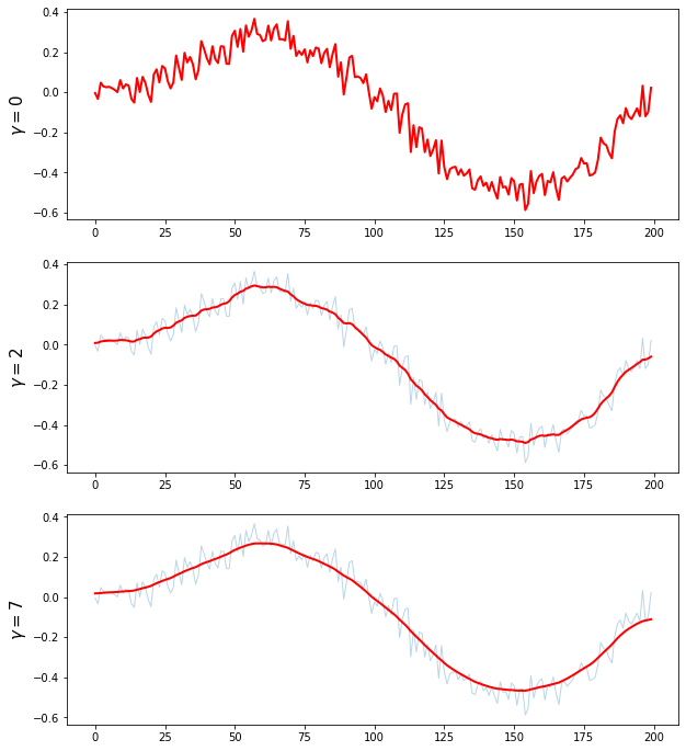
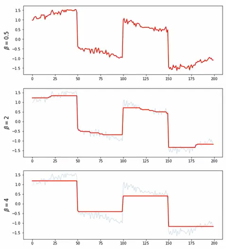
- Signal with Sharp Transition + Noise
- 대부분 smoothing하지만 일부분이 급격하게 달라지는 그래프에 대한 처리
- L2보다 L1이 처리를 더 잘하는 것으로 확인할 수 있다.
# Signal with sharp Transition * Noise
n = 200
t = np.arange(n).reshape(-1,1)
exact = np.vstack([np.ones([50,1]), -np.ones([50,1]), np.ones([50,1]), -np.ones([50,1])])
x = exact + 0.5*np.sin((2*np.pi/n)*t)
x_cor = x + 0.1*np.random.randn(n,1)
plt.figure(figsize = (10,8))
plt.subplot(2,1,1)
plt.plot(t,x)
plt.ylim([-2.0, 2.0])
plt.ylabel('signal', fontsize = 15)
plt.subplot(2,1,2)
plt.plot(t, x_cor, linewidth = 1)
plt.ylabel('corrupted signal', fontsize = 15)
plt.xlabel('x', fontsize = 15)
plt.show()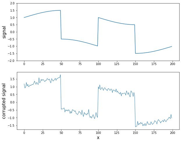
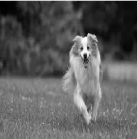
- 사진 smoothing
import cv2
imbw = cv2.imread('사진경로',0)
row = 150
col = 150
resized_imbw = cv2.resize(imbw,(row,col))
plt.figure(figsize = (8,8))
plt.imshow(resized_imbw, 'gray')
plt.axis('off')
plt.show()

n = row*col
imbws = resized_imbw.reshape(-1,1)
beta = 1500
x = cvx.Variable([n,1])
obj = cvx.Minimize(cvx.norm(x[1:n] - x[0:n-1],1))
const = [cvx.norm(x - imbws, 2) <= beta]
prob = cvx.Problem(obj, const).solve()
imbwr = x.value.reshape(row,col)
plt.figure(figsize = (8,8))
plt.imshow(imbwr, 'gray')
plt.axis('off')
plt.show()
- 예시 결과

< 추가 실습 >
- Python
https://kyudon.tistory.com/279
- R